2. Quickstart
2.1. Overview
Pyret is a Python package that provides tools for analyzing stimulus-evoked
neurophysiology data. The project grew out of work in a retinal neurophsyiology
and computation lab (hence the name), but its functionality should be applicable
to any neuroscience work in which you wish to characterize how neurons behave
in response to an input.
Pyret’s functionality is broken into modules.
stimulustools: Functions for manipulating input stimuli.spiketools: Tools to characterize spikes.filtertools: Tools to estimate and characterize linear filters fitted to neural data.nonlinearities: Classes for estimating static nonlinearities.visualizations: Functions to visualize responses and fitted filters/nonlinearities.
Pyret works on Python3.4+ and Python2.7.
2.2. Demo
2.2.1. Importing pyret
Let’s explore how pyret might be used in a very common analysis pipeline. First, we’ll
import the relevant modules.
>>> import pyret
>>> import numpy as np
>>> import matplotlib.pyplot as plt
For this demo, we’ll be using data from a retinal ganglion cell (RGC), whose spike times were recorded using a multi-electrode array. (Data courtesy of Lane McIntosh.) We’ll load the stimulus used in the experiment, as well as the spike times for the cell.
The data is stored in the GitHub repository, in both HDF5 and NumPy’s native .npz formats.
The following code snippets show how to download and load the data in those formats,
respectively. Note that using data in the HDF5 format imposes the additional dependency of
the h5py package, which is available on PyPI.
2.2.2. Loading data from HDF5
To download the data in HDF5 format, use the shell command:
$ wget https://github.com/baccuslab/pyret/raw/master/docs/tutorial-data.h5
To use curl instead of wget, run:
$ curl -L -o tutorial-data.h5 https://github.com/baccuslab/pyret/raw/master/docs/tutorial-data.h5
To load the data, back in the Python shell, run:
>>> data_file = h5py.File('tutorial-data.h5', 'r')
>>> spikes = data_file['spike-times']  # Spike times for one cell
>>> stimulus = data_file['stimulus'].value.astype(np.float64)
>>> frame_rate = data_file['stimulus'].attrs.get('frame-rate')
2.2.3. Loading data from .npz
To download and the data in the .npz file format, use the following command:
$ wget https://github.com/baccuslab/pyret/raw/master/docs/tutorial-data.npz
Or, using curl:
$ curl -L -o tutorial-data.npz https://github.com/baccuslab/pyret/raw/master/docs/tutorial-data.npz
Then, in the Python shell, load the data with:
>>> arrays = np.load('tutorial-data.npz')
>>> spikes, stimulus, frame_rate = arrays['spikes'], arrays['stimulus'].astype(np.float64), arrays['frame_rate'][0]
2.2.4. Estimating firing rates
The stimulus is a spatio-temporal gaussian white noise checkboard, with shape (time, nx, ny).
Each spatial position is drawn independently from a normal distribution on each
temporal frame. We will z-score the stimulus, and create a time-axis for it, to reference
the spike times for this cell to the frames of the stimulus.
>>> stimulus -= stimulus.mean()
>>> stimulus /= stimulus.std()
>>> time = np.arange(stimulus.shape[0]) * frame_rate
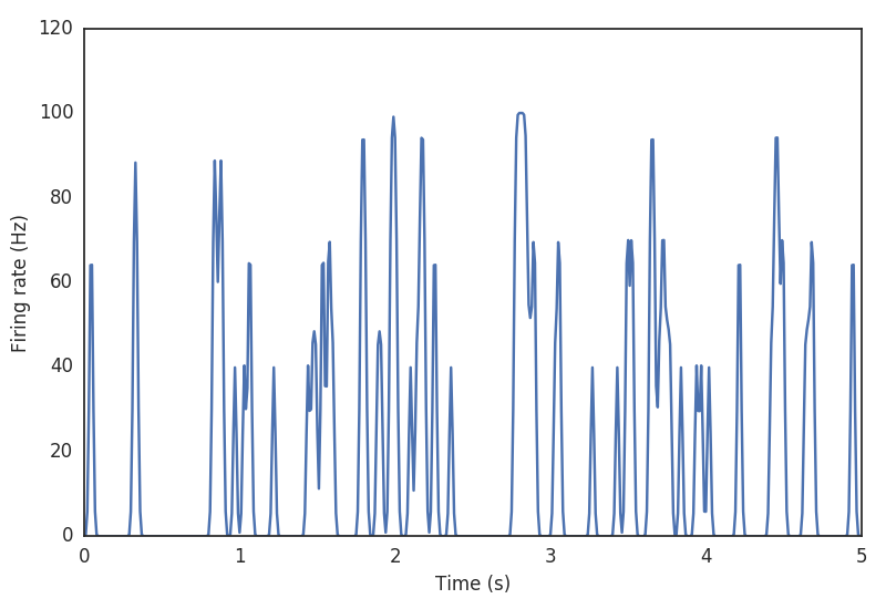
To begin, let’s look at the spiking behavior of the RGC. We’ll create a peri-stimulus time histogram, by binning the spike times and smoothing a bit. This is an estimate of the firing rate of the RGC over time.
>>> binned = pyret.spiketools.binspikes(spikes, time)
>>> rate = pyret.spiketools.estfr(binned, time)
>>> plt.plot(time[:500], rate[:500])
>>> plt.xlabel('Time (s)')
>>> plt.ylabel('Firing rate (Hz)')
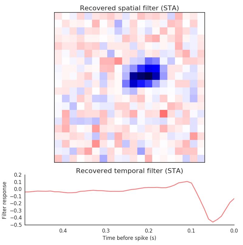
2.2.5. Estimating a receptive field
One widely-used and informative description of the cell is its receptive field. This is a linear approximation to the function of the cell, and captures the average visual feature to which it responds. Because our data consists of spike times, we’ll compute the spike-triggered average (STA) for the cell.
>>> filter_length_seconds = 0.5  # 500 ms filter
>>> filter_length = int(filter_length_seconds / frame_rate)
>>> sta, tax = pyret.filtertools.sta(time, stimulus, spikes, filter_length)
>>> fig, axes = pyret.visualizations.plot_sta(tax, sta)
>>> axes[0].set_title('Recovered spatial filter (STA)')
>>> axes[1].set_title('Recovered temporal filter (STA)')
>>> axes[1].set_xlabel('Time relative to spike (s)')
>>> axes[1].set_ylabel('Filter response')
Important
It is common to hear the terms “STA”, “linear filter”, and “receptive field”
used interchangeably. However, this is technically incorrect. The STA is an
unbiased estimate of the time-reverse of a best-fitting linear filter (in
the least-squares sense), assuming the stimulus is uncorrelated. If the
stimulus contains correlations, those will appear in the arrays returned by
both filtertools.sta and filtertools.revcorr. As Gaussian white
noise, which is uncorrelated, is an exceedingly common stimulus, practioners
often loosely refer to the STA as the linear filter, keeping the time-reversing
process implicit. The pyret methods and docstrings strive for the maximal
amount of clarity when refering to these objects, and the documentation should
be heeded about whether a filter or STA is expected.
2.2.6. Estimating a nonlinearity
While the STA gives a lot of information, it is not the whole story. Real RGCs are definitely not linear. One common way to correct for this fact is to fit a single, time-invariant (static), point-wise nonlinearity to the data. This is a mapping between the linear response to the real spiking data; in other words, it captures the difference between how the cell would response if it were linear and how the cell actually responds.
The first step in computing a nonlinearity is to compute how the recovered linear filter responds to the input stimulus. This is done via convolution of the linear filter with the stimulus.
>>> pred = pyret.filtertools.linear_response(sta[::-1], stimulus)
>>> stimulus.shape
(30011, 20, 20)
>>> pred.shape
(30011,)
Important
Note here that we’re flipping the STA before passing it to the
linear_response function. This function expects a true linear filter,
while the arrays returned by sta and revcorr are reverse-
correlations. This must be flipped along the time (zero-th) axis
to arrive at a filter.
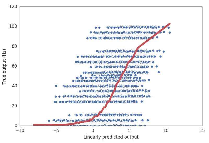
We can get a sense for how poor our linear prediction is, simply by plotting the predicted versus the actual response at each time point.
>>> plt.plot(pred, rate, linestyle='none', marker='o', mew=1, mec='w')
>>> plt.xlabel('Linearly predicted output')
>>> plt.ylabel('True output (Hz)')
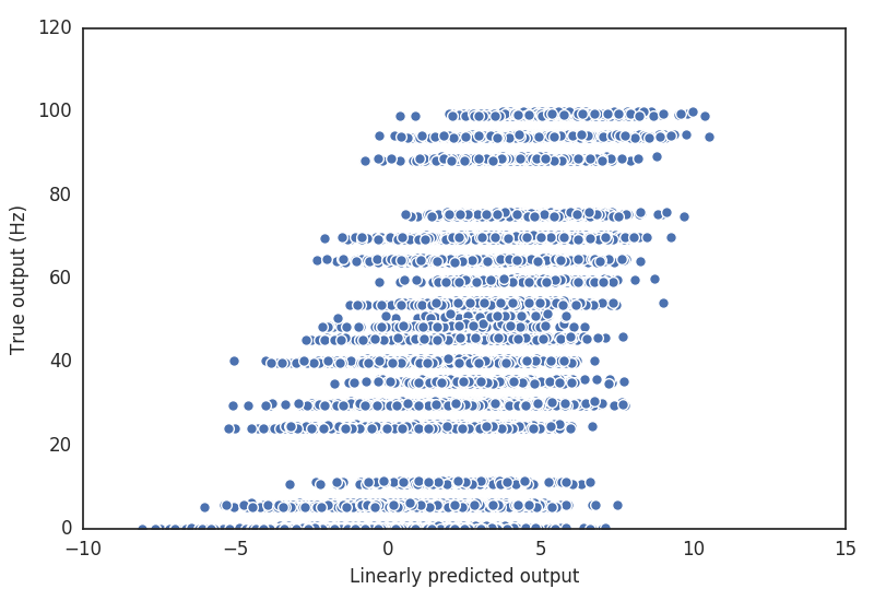
It’s clear that there is at least some nonlinear behavior in the cell. For one thing, firing rates can never be negative, but our linear prediction definitely is.
pyret contains several classes for fitting nonlinearities to data. The simplest is
the Binterp class (a portmanteau of “bin” and “interpolate”), which computes the
average true output in specified bins along the input axis. It uses variable-sized
bins, so that each bin has roughly the same number of data points.
>>> nbins = 50
>>> binterp = pyret.nonlinearities.Binterp(nbins)
>>> binterp.fit(pred, rate)
>>> nonlin_range = (pred.min(), pred.max())
>>> binterp.plot(nonlin_range, linewidth=5, label='Binterp')  # Plot nonlinearity over the given range
One can also fit sigmoidal nonlinearities, or a nonlinearity using a Gaussian process (which has some nice advantages, and returns errorbars automatically). More information about these can be found in the full documentation.
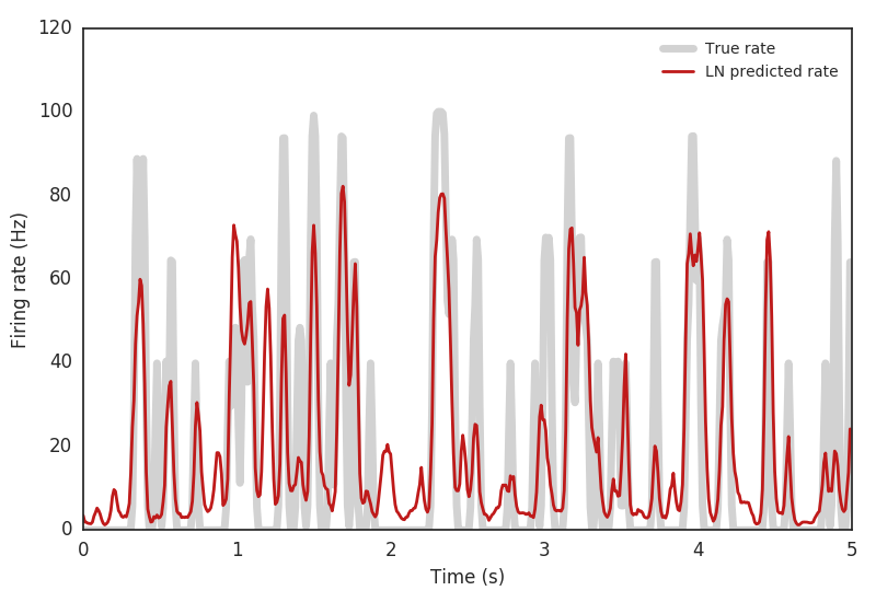
We can now compare how well the full LN model captures the cell’s response characteristics.
>>> predicted_rate = binterp.predict(pred)
>>> plt.figure()
>>> plt.plot(time[:500], rate[:500], linewidth=5, color=(0.75,) * 3, alpha=0.7, label='True rate')
>>> plt.plot(time[:500], predicted_rate[:500], linewidth=2, color=(0.75, 0.1, 0.1), label='LN predicted rate')
>>> plt.legend()
>>> plt.xlabel('Time (s)')
>>> plt.ylabel('Firing rate (Hz)')
>>> np.corrcoef(rate, predicted_rate)[0, 1] # Correlation coefficient on training data
0.70315310866999448